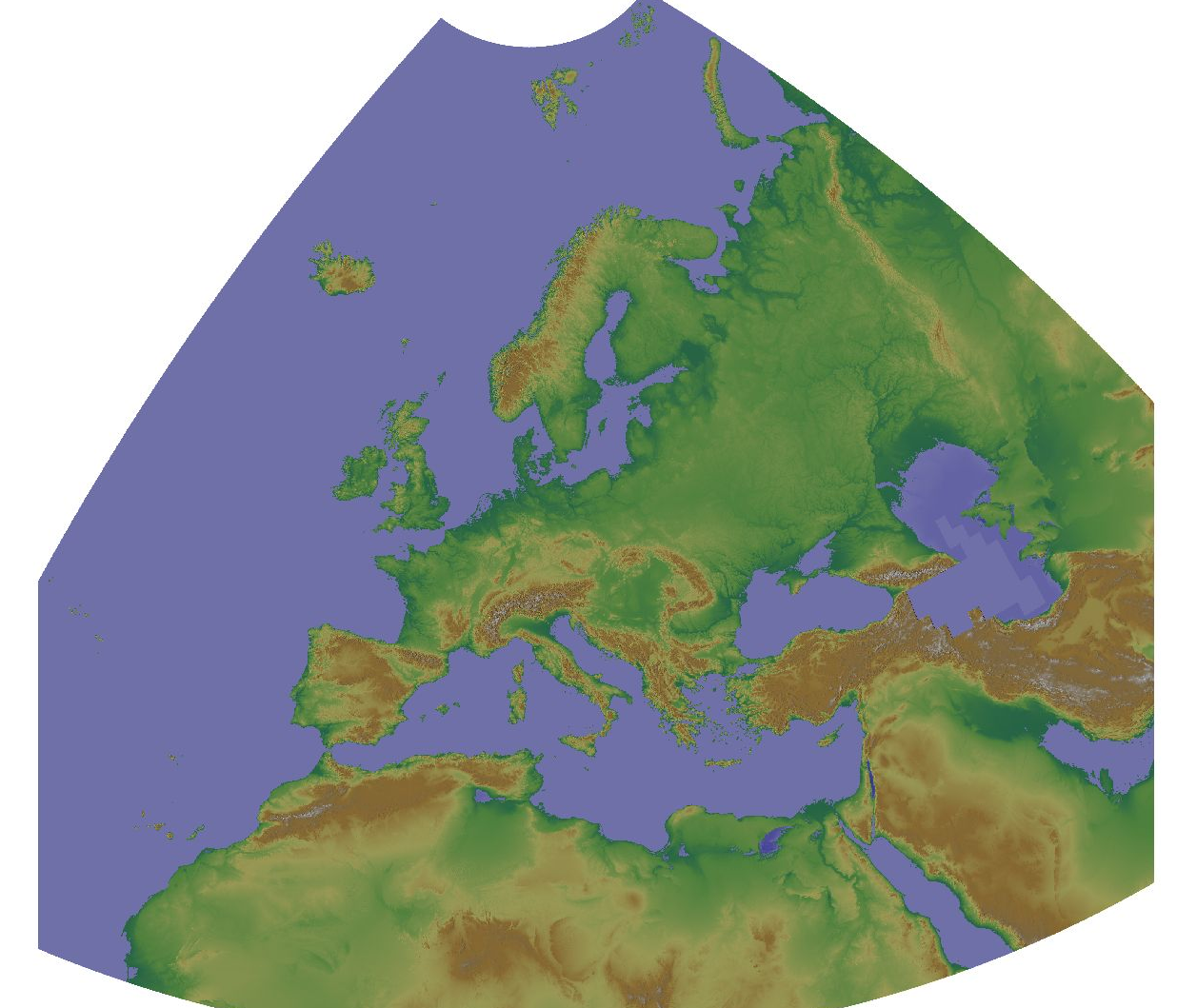
The Copernicus DEM is a Digital Surface Model (DSM) which represents the surface of the Earth including buildings, infrastructure and vegetation. The original GLO-30 provides worldwide coverage at 30 meters (refers to 10 arc seconds). Note that ocean areas do not have tiles, there one can assume height values equal to zero. Data is provided as Cloud Optimized GeoTIFFs. Note that the vertical unit for measurement of elevation height is meters. The Copernicus DEM for Europe at 1000 meter resolution (EU-LAEA projection) in COG format has been derived from the Copernicus DEM GLO-30, mirrored on Open Data on AWS, dataset managed by Sinergise (https://registry.opendata.aws/copernicus-dem/). Processing steps: The original Copernicus GLO-30 DEM contains a relevant percentage of tiles with non-square pixels. We created a mosaic map in https://gdal.org/drivers/raster/vrt.html format and defined within the VRT file the rule to apply cubic resampling while reading the data, i.e. importing them into GRASS GIS for further processing. We chose cubic instead of bilinear resampling since the height-width ratio of non-square pixels is up to 1:5. Hence, artefacts between adjacent tiles in rugged terrain could be minimized: gdalbuildvrt -input_file_list list_geotiffs_MOOD.csv -r cubic -tr 0.000277777777777778 0.000277777777777778 Copernicus_DSM_30m_MOOD.vrt In order to reproject the data to EU-LAEA projection while reducing the spatial resolution to 1000 m, bilinear resampling was performed in GRASS GIS (using r.proj) and the pixel values were scaled with 1000 (storing the pixels as Integer values) for data volume reduction. In addition, a hillshade raster map was derived from the resampled elevation map (using r.relief, GRASS GIS). Eventually, we exported the elevation and hillshade raster maps in Cloud Optimized GeoTIFF (COG) format, along with SLD and QML style files.

Temperature time series with high spatial and temporal resolutions are important for several applications. The new MODIS Land Surface Temperature (LST) collection 6 provides numerous improvements compared to collection 5. However, being remotely sensed data in the thermal range, LST shows gaps in cloud-covered areas. With a novel method [1] we fully reconstructed the daily global MODIS LST products MOD11A1/MYD11A1 (spatial resolution: 1 km). For this, we combined temporal and spatial interpolation, using emissivity and elevation as covariates for the spatial interpolation. Here we provide a time series of these reconstructed LST data aggregated as daily LST maps at overpass time (approx: 01:30 am, 10:30am, 1:30pm 10:30pm). [1] Metz M., Andreo V., Neteler M. (2017): A new fully gap-free time series of Land Surface Temperature from MODIS LST data. Remote Sensing, 9(12):1333. DOI: http://dx.doi.org/10.3390/rs9121333 The data are provided in GeoTIFF format. The Coordinate Reference System (CRS) is identical to the MOD11A1/MYD11A1 product (Sinusoidal) as provided by NASA. In WKT as reported by GDAL: PROJCRS["unnamed", BASEGEOGCRS["Unknown datum based upon the custom spheroid", DATUM["Not specified (based on custom spheroid)", ELLIPSOID["Custom spheroid",6371007.181,0, LENGTHUNIT["metre",1, ID["EPSG",9001]]]], PRIMEM["Greenwich",0, ANGLEUNIT["degree",0.0174532925199433, ID["EPSG",9122]]]], CONVERSION["unnamed", METHOD["Sinusoidal"], PARAMETER["Longitude of natural origin",0, ANGLEUNIT["degree",0.0174532925199433], ID["EPSG",8802]], PARAMETER["False easting",0, LENGTHUNIT["Meter",1], ID["EPSG",8806]], PARAMETER["False northing",0, LENGTHUNIT["Meter",1], ID["EPSG",8807]]], CS[Cartesian,2], AXIS["easting",east, ORDER[1], LENGTHUNIT["Meter",1]], AXIS["northing",north, ORDER[2], LENGTHUNIT["Meter",1]]] Acknowledgments: We are grateful to the NASA Land Processes Distributed Active Archive Center (LP DAAC) for making the MODIS LST data available. The dataset is based on MODIS Collection V006. Meaning of pixel values: The pixel values are coded in Kelvin * 50 Data type: raster, UInt16 Spatial resolution: 926.62543314 m Spatial extent Sinusoidal (W, S, E, N): 0, 4447802.079066, 2223901.039533, 6671703.118599 Spatial extent in EPSG:4326 (W, S, E, N): 0, 40, 40, 60

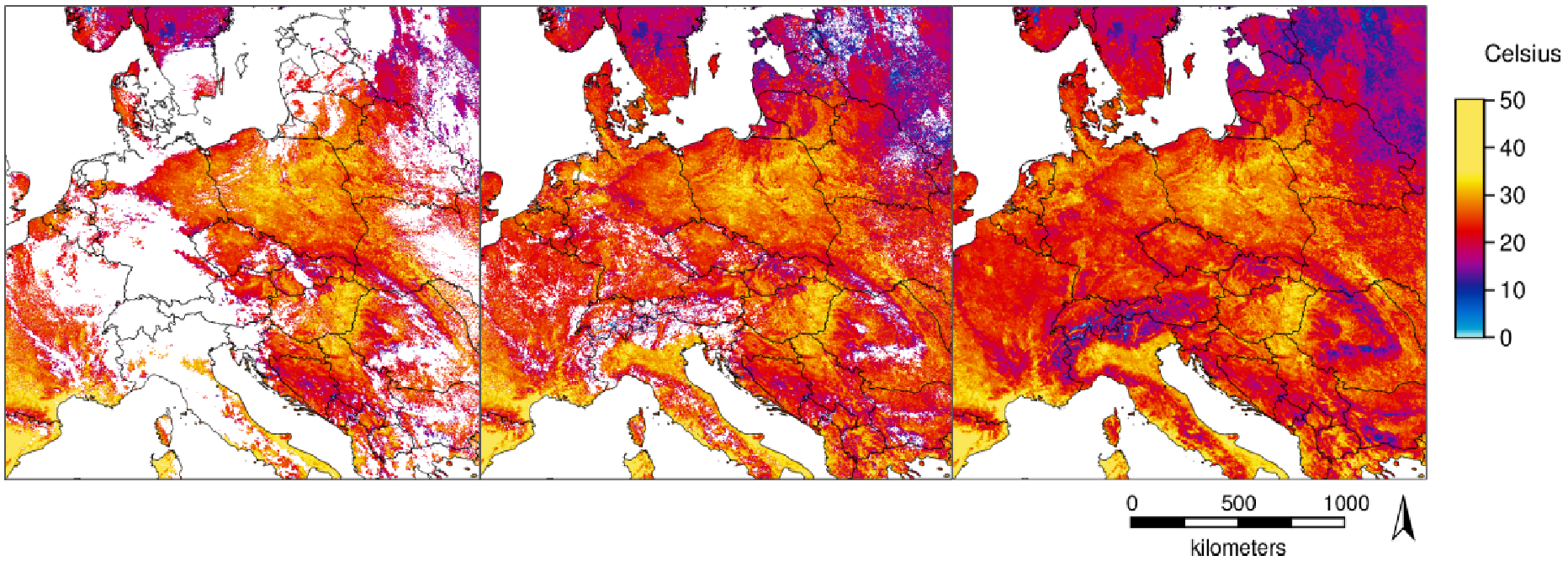
Northern Italy Land Surface Temperature 1km daily Celsius gap-filled datasetLST daily avg, 2010 - 2018, reconstructed format: GRASS GIS raster format ZLIB compressed stored as a GRASS GIS 7 location/mapset Projection: EU LAEA (EPSG:3035)Reference: Metz, M.; Andreo, V.; Neteler, M. A New Fully Gap-Free Time Series of Land Surface Temperature from MODIS LST Data. Remote Sens. 2017, 9, 1333. https://doi.org/10.3390/rs9121333

This global accessibility map enumerates land-based travel time to the nearest densely-populated area for all areas between 85 degrees north and 60 degrees south for a nominal year 2015. Densely-populated areas are defined as contiguous areas with 1,500 or more inhabitants per square kilometer or a majority of built-up land cover types coincident with a population centre of at least 50,000 inhabitants. This map was produced through a collaboration between the University of Oxford Malaria Atlas Project (MAP), Google, the European Union Joint Research Centre (JRC), and the University of Twente, Netherlands. The underlying datasets used to produce the map, include roads (comprising the first ever global-scale use of Open Street Map and Google roads datasets), railways, rivers, lakes, oceans, topographic conditions (slope and elevation), landcover types, and national borders. These datasets were each allocated a speed or speeds of travel in terms of time to cross each pixel of that type. The datasets were then combined to produce a “friction surface”, a map where every pixel is allocated a nominal overall speed of travel based on the types occurring within that pixel. Least-cost-path algorithms (running in Google Earth Engine and, for high-latitude areas, in R) were used in conjunction with this friction surface to calculate the time of travel from all locations to the nearest city (by travel time). Cities were determined using the high-density-cover product created by the Global Human Settlement Project. Each pixel in the resultant accessibility map thus represents the modeled shortest time from that location to a city. Full Citation D.J. Weiss, A. Nelson, H.S. Gibson, W. Temperley, S. Peedell, A. Lieber, M. Hancher, E. Poyart, S. Belchior, N. Fullman, B. Mappin, U. Dalrymple, J. Rozier, T.C.D. Lucas, R.E. Howes, L.S. Tusting, S.Y. Kang, E. Cameron, D. Bisanzio, K.E. Battle, S. Bhatt, and P.W. Gething. A global map of travel time to cities to assess inequalities in accessibility in 2015. (2018). Nature. doi:10.1038/nature25181.

Temperature time series with high spatial and temporal resolutions are important for several applications. The new MODIS Land Surface Temperature (LST) collection 6 provides numerous improvements compared to collection 5. However, being remotely sensed data in the thermal range, LST shows gaps in cloud-covered areas. With a novel method [1] we fully reconstructed the daily global MODIS LST products MOD11C1 and MYD11C1 (spatial resolution: 3 arc-min, i.e. approximately 5.6 km at the equator). For this, we combined temporal and spatial interpolation, using emissivity and elevation as covariates for the spatial interpolation. Here we provide a time series of these reconstructed LST data aggregated as monthly average, minimum and maximum LST maps. [1] Metz M., Andreo V., Neteler M. (2017): A new fully gap-free time series of Land Surface Temperature from MODIS LST data. Remote Sensing, 9(12):1333. DOI: http://dx.doi.org/10.3390/rs9121333 The data available here for download are the reconstructed global MODIS LST products MOD11C1/MYD11C1 at a spatial resolution of 3 arc-min (approximately 5.6 km at the equator; see https://lpdaac.usgs.gov/dataset_discovery/modis/modis_products_table), aggregated to monthly data. The data are provided in GeoTIFF format. The Coordinate Reference System (CRS) is identical to the MOD11C1/MYD11C1 product as provided by NASA. In WKT as reported by GDAL: GEOGCS["Unknown datum based upon the Clarke 1866 ellipsoid", DATUM["Not specified (based on Clarke 1866 spheroid)", SPHEROID["Clarke 1866",6378206.4,294.9786982138982, AUTHORITY["EPSG","7008"]]], PRIMEM["Greenwich",0], UNIT["degree",0.0174532925199433]] Acknowledgments: We are grateful to the NASA Land Processes Distributed Active Archive Center (LP DAAC) for making the MODIS LST data available. The dataset is based on MODIS Collection V006. File name abbreviations: avg = average of daily averages min = minimum of daily minima max = maximum of daily maxima Meaning of pixel values: The pixel values are coded in degree Celsius * 100 (hence, to obtain °C divide the pixel values by 100.0).